Overview

Every year, farmers count vast amounts of seedlings for insurance reasons and to calculate replanting requirements. In research trials, the calculation of tassels gives an estimate for the percentage of emerging seedlings. Consequently, later in the season, farmers tend to count tassels as a better prediction of yield.#nbsp;

The seedling counting technique has been in use for a few years already. However, the process has never been as quick as it is now with ATLAS, an AI-powered platform enabling storage and analysis of geospatial data.

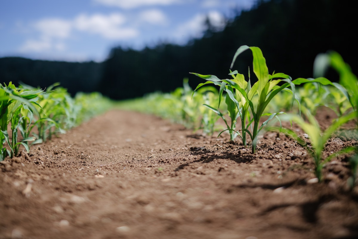
This article explains how to utilize RGB imagery from drones to count vast amounts of seedlings of various plants in the field. We used images of a cornfield, detecting a total of 36,582 objects in the test area of 0.74Ha. The map had a GSD of 1cm, which was more than sufficient for our task. Overall, the project took 25 minutes of manual data annotation and three hours of cloud processing in ATLAS.

Workflow

In our case, we already have an orthomosaic stitched in Pix4D Mapper. The uploading process to ATLAS is straightforward and will not be covered here. So, what do we see when the map is in ATLAS?

Only a map is visible, with no annotations. The next step is to press the “New object search” button in the upper toolbar. A dialog box then appears where we can enter the name of the object of interest.

In the “Search for” field, we can either create a new object name or pick from existing objects. As there was no existing object for corn seedlings in our case, we click on “New object of interest”.

We can then give a “corn-seedling” name to our object and move to the next important stage – manual annotation. This consists of two steps:

• annotate “Training samples” - in our case this means visible footprints of green seedlings
• annotate “Training areas” - these are used by ATLAS for AI training. The area shows ATLAS what is part of the object of interest (training sample) and what is background. Therefore, the only rule to remember is that inside the training areas, all objects of interest should be marked as training samples. Not following this rule could lead to missing objects in the generated results.

To annotate training samples and training areas, we use the same drawing tools (1) from the upper toolbar. The currently selected item in the right panel (2) defines the context.

The resulting annotation may look like the picture below:

The dashed polygon defines the training area and all seedlings inside this polygon have proper annotation.

Let us define what “proper annotation” actually means. It is highly recommended that you follow object contours as close as possible. There are three main tools on the annotation toolbar: circle, polygon, and rectangle. We can typically achieve the best results with a polygon, while circles and rectangles often seize too much background, which may lead to excessive false positives. However, circles can be very handy for palm annotation.

When an annotation is completed, we press either “Continue” in the window or “New object search” again, which opens the following dialog box:

The next step is to specify where to make an automated object search. ATLAS has two options:

• “Detect on entire map”, which is good when you are confident in detector quality.
• “Detect on working area”, which allows you to specify the region for test detection. It is also useful when there are obvious regions where no object of interest can exist. We can specify only the field boundary, which has plants and leave out the scope an empty area. This may save hours of processing for large surveys.

In this particular example, we specify the working area, the properties of which are displayed by the right panel. To draw the boundary, we can use all of the same tools from the upper toolbar, with the working area being shown via a white dashed line.

In the property panel on the right, we can see the area size and number of objects inside it. After we finish defining the working area, we either press “Continue” in the dialog box or “New object search” in the upper toolbar.

Once the new dialog box appears, make the final check:

• Search for: “corn-seedlings”
• Where to search: “Detect on working area”

Each seedling should be annotated as a simple (convex) polygon. This is why we choose “Simple objects” for the desired object shape.

Once all is prepared, press “Find objects”. The detection process can take a while and you will receive an email notification when it is complete.

Inspect detection results: If the results are good, they can be used for counting or exported as GeoJSON.

If the results are not perfect, check your annotation. There are several common reasons for poor performance:

• Not all training samples are annotated within the training area.
• Background objects are annotated as objects of interest.
• Too few annotations.

Review your annotation, fix it and repeat the search. To improve detection results, we recommend that you select a previously trained detector for this object type. This will prevent ATLAS from having to learn from scratch by reusing knowledge obtained during the previous detection.